Why Workforce Forecasts Underestimate Staffing Risk

A workforce forecast can be mathematically correct and still give managers the wrong impression.

Suppose a contact center expects 100 calls on Tuesday morning. The model produces its best estimate, staffing is planned around it, and the dashboard says everything should be fine. Then Tuesday arrives and 130 calls come in. The queue falls behind, service levels drop, and the manager asks the obvious question: why did the system say we were covered?

The problem is not necessarily the point forecast. Forecasts will always be wrong to some degree. The deeper problem is that many forecasting systems underestimate how wrong they might be.

At Soon, we are building a simulation layer that does not only ask, "What volume do we expect?" It also asks, "What could realistically happen around that forecast, and how often would the current schedule still hold up?"

Two ideas matter enormously if that simulation is going to be useful: over-dispersion and correlated forecast errors. The names sound technical. The operating reality is simple. Some queues are burstier than a tidy model expects, and bad periods often arrive together.

How wrong are your forecasts, really?

When a simulator plays out thousands of possible future weeks, it has to decide how much randomness to add around the forecast. A textbook assumption might say that when you forecast 100 calls, most outcomes should land close to 100. Maybe 94 calls, 103 calls, or 108 calls.

That can be reasonable in a stable operation. Real contact centers are rarely that tidy. A marketing email goes out earlier than expected. A payment flow fails. Heavy rain changes customer behavior. A product update creates confusion. Another department contacts thousands of customers without telling operations. Suddenly, 100 expected calls becomes 130.

The surprising thing is not that these events happen. Everyone working in operations knows they happen. The surprising thing is how often forecasting software behaves as if they barely happen at all.

The difference between theory and receipts

Imagine two planners discussing the same Tuesday. The first says, "The model considered this extremely unlikely." The second opens the historical data and says, "But something like this happened twice last month."

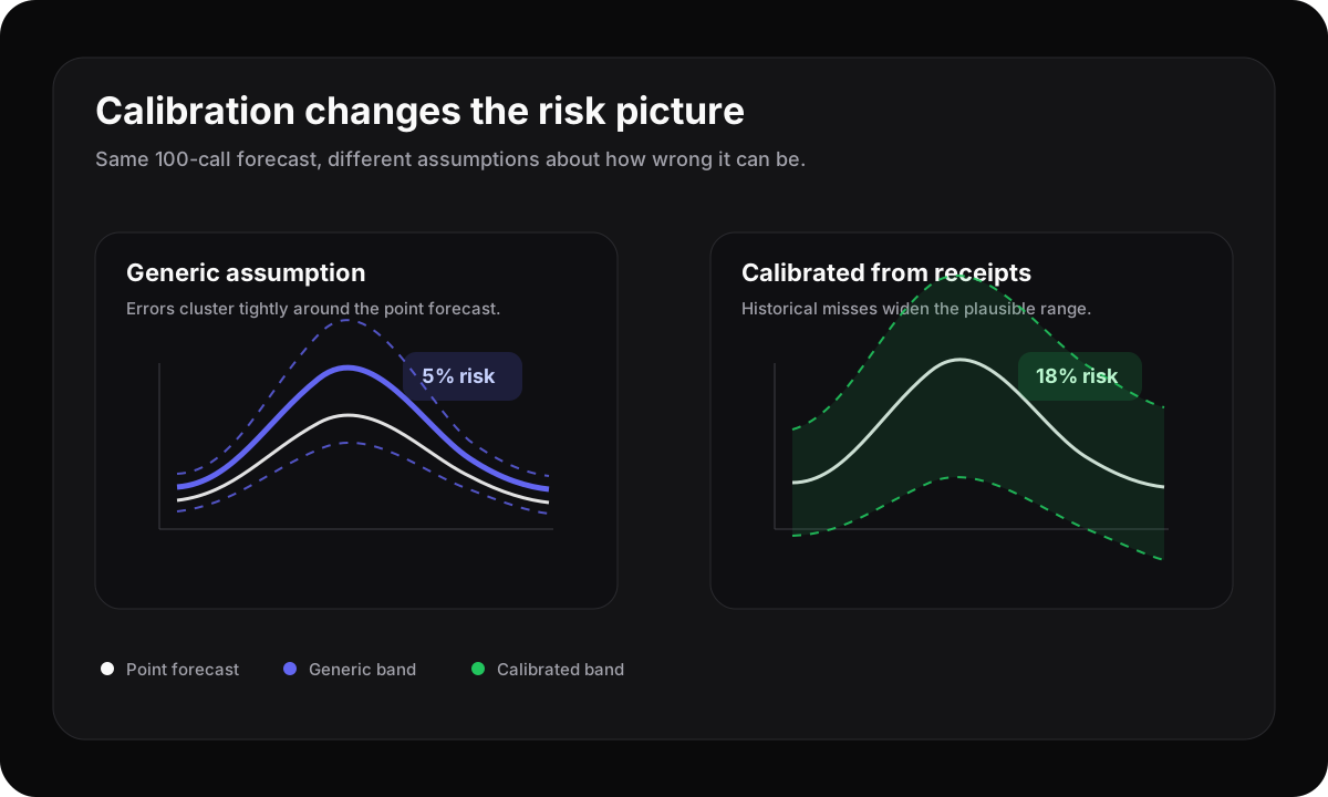
That gap is what calibration is designed to close. Instead of using a generic statistical assumption, the simulator should learn from the customer's own forecast history. For each historical interval, compare what the system forecast with what actually happened. The difference is the residual, which is just another name for forecast error.

If the forecast was 100 and actual demand was 115, the residual is +15. If the forecast was 100 and actual demand was 90, the residual is -10. Over time, those differences reveal the real personality of an operation. Some queues are stable. Some are quiet most of the time but occasionally explode. Some miss more often on Mondays, during billing runs, or after campaigns.

By measuring those misses, a simulator can generate scenarios that look like the customer's operation, not like an idealized textbook version of it.

Why frozen forecasts matter

Calibration only works when old forecasts are preserved. A system should not quietly replace yesterday's forecast with a newer, improved version and then compare that revised forecast with reality. That is like predicting yesterday's weather after looking out the window.

Past forecasts need to stay frozen. They are the receipts. They show what the business genuinely believed at the time and how reality differed from that belief.

Given how this queue has behaved in the past, how large are its forecast errors likely to be in the future?

That is a much more useful question than asking whether a single point forecast looks plausible.

The practical difference

An uncalibrated simulator might say there is a 5% chance Tuesday goes badly. A calibrated simulator might say the chance is 18% because this queue has historically missed its forecast by that amount.

The second answer may be less comfortable. It is also more useful. Managers do not need optimistic numbers. They need numbers that match lived experience.

Bad mornings often become bad days

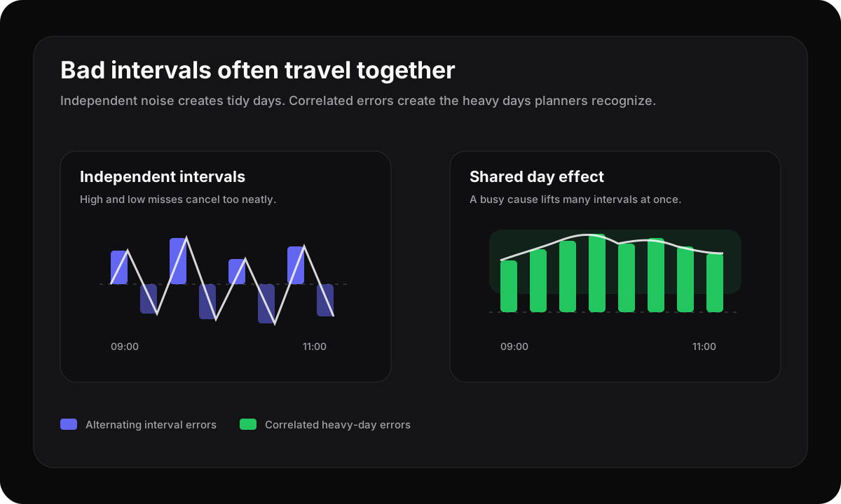
There is another subtle problem in many simulations. Imagine the forecast is split into 15-minute intervals and the simulator adds a little randomness to each interval independently. At 09:00, volume comes in much higher than expected. At 09:15, it comes in lower. At 09:30, it is slightly higher. At 09:45, it is lower again. Across the morning, the errors conveniently cancel each other out.

The simulated day looks manageable. Real life is often less polite.

The heavy-day effect

At 09:00, the first warning appears. The queue is already above forecast. A planner may initially assume it is a short spike. But at 09:15, the volume remains high. At 09:30, it is still high. By lunch, everyone understands this is not a bad interval. It is a bad day.

The cause may be invisible to the forecast but obvious in hindsight. A campaign launched. A supplier had an outage. A letter landed on thousands of doormats. An app release confused customers. The same underlying event affects many intervals at once.

That means forecast errors are often correlated. When one interval is unusually busy, nearby intervals are more likely to be unusually busy too.

Simulating the kind of day

To represent this, the simulator needs more than independent noise for every interval. It also needs a shared day-level effect. You can think of it as rolling one die to determine the overall character of the day: quiet, normal, or heavy. Smaller interval-level variations are then added on top.

This produces scenarios that look much more like real operations. A heavy day remains heavy for several hours. A quiet day may stay below forecast. A sudden event can affect the complete shape of demand instead of disappearing after 15 minutes.

When every interval is simulated independently, positive and negative misses cancel too easily. The result is a world where staffing problems are brief, isolated, and unusually convenient. That can make a simulation say you will achieve service level on 95% of days. Once whole-day effects are represented, the answer may become 80%. No individual forecast number changed. The simulation simply became capable of producing an entire difficult day.

This is what planners already call a safety buffer

Workforce planners may not ask for over-dispersion or correlated residuals. They do deal with the consequences every week. The common workaround is simple: add another 10% to be safe.

That extra 10% is a human attempt to compensate for uncertainty the software has failed to represent. Sometimes it works. Sometimes it creates unnecessary staffing cost. Sometimes it is not nearly enough.

The problem is that the percentage is usually based on experience, instinct, and recent pain. It may be applied equally across queues that behave very differently. Calibration turns that instinct into something measurable.

• Queue A is highly stable and needs only a modest buffer.
• Queue B is unpredictable on Mondays.
• Queue C regularly experiences whole-day demand shocks.
• Queue D has become more predictable as the forecasting model has improved.

The safety margin becomes specific to the operation. It can also be explained. A planner can tell a finance director, "We are not adding 15% because it feels safer. We are staffing for a risk level derived from our historical forecast errors."

Why this matters for Monte Carlo simulation

Monte Carlo simulation sounds sophisticated, but the basic idea is simple. The system creates many plausible versions of the future and tests the schedule against each one.

For example, it may simulate 2,000 possible weeks and calculate how often service level is achieved, how often occupancy becomes unsafe, how often demand exceeds staffing, which intervals are most vulnerable, and how much extra capacity would reduce risk.

But a simulation is only as honest as the scenarios it generates. If the scenarios are too smooth, too independent, or too close to the forecast, the output becomes systematically optimistic. The dashboard may show a precise number such as 11% risk of missing service level, but precision is not the same as accuracy.

Without calibration, that 11% may reflect the simulator's assumptions more than the operation's reality. A risk number that looks scientific but consistently understates risk is worse than no risk number at all. It encourages decisions based on false confidence.

With calibration, the number has a clearer meaning: based on how this operation's forecasts have historically differed from reality, schedules like this failed in about 11% of simulated scenarios. That is a number managers can begin to trust.

How we are building it at Soon

We are adding calibration directly into Soon's simulation workflow. For each forecast stream, the system will use historical forecast-versus-actual data to estimate how widely actual demand tends to vary around the forecast, how often large misses occur, how much forecast errors persist across intervals, and how strongly a busy interval predicts a busy day.

The simulator can then create scenarios that match the behavior of that specific stream. An hourly back-office queue and a 15-minute customer support queue may receive very different uncertainty profiles. That is intentional. Different operations should produce different risks.

This is where forecasting, simulation, and intraday management start to work as one loop. The forecast gives the plan a center of gravity. Simulation shows how the plan behaves when reality moves. Intraday workflows help teams respond when the day starts proving the forecast wrong.

What happens when there is not enough history?

Calibration requires enough historical overlap between forecasts and actual demand. As a practical starting point, we expect roughly four or more weeks of usable forecast-versus-actual data per stream before relying heavily on customer-specific calibration.

When that history is not available yet, the simulation still works. It falls back to a broader uncertainty model based on forecast bands and default assumptions. As more history accumulates, the customer-specific calibration becomes more reliable.

That matters for new customers. They do not need to wait months before using simulation. The system can provide an initial risk estimate immediately and become more personalized over time. Migrating historical forecast and actual data into durable storage is therefore not just a technical task. It gives the simulation its memory.

The real product is trust

A forecast is not a promise. A simulation should not pretend that it is. The purpose of a risk model is not to make the schedule look safe. It is to show how the schedule behaves when reality refuses to follow the plan.

That means acknowledging that contact centers are burstier than textbook models suggest, forecast errors often persist across a complete day, every queue has a different uncertainty profile, and historical forecast mistakes are valuable information.

Once those effects are represented honestly, a planner can move beyond, "The forecast says we should be fine." They can start saying, "Given the uncertainty we have actually experienced, this schedule has an 89% chance of achieving the target."

That is a more defensible decision. In workforce planning, trust does not come from predicting the future perfectly. It comes from being honest about how unpredictable the future really is.